This is my last blog post on the persistent vector! In the previous blog posts, we’ve looked at how to do efficient immutable updates on the vector, we’ve looked at indexing, how the tail works, and how transients can be implemented. Now we’re only left with two big questions: Why a branching factor of 32, and what is “effectively constant time”? We will also have a quick peek into its memory consumption.

If you’re very interested in all the small details related to this blog post, you should have a look at my blog post on Persistent Vector Performance. It contains a lot of tips for practitioners on how to improve its performance as well.

Why 2⁵?

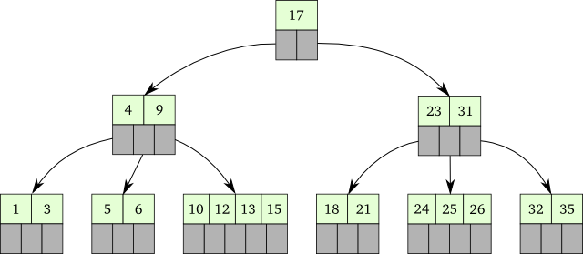
The B-tree is a data structure which acts and behaves in very much the same way as a balanced binary tree: Assuming a lookup takes constant time, both have the same asymptotic running time. However, when used for storing data on disk, it becomes much more efficient than any binary tree. Why? Because reading from disk is slow, but once you start reading from it, it’s very cheap to read “bulks” of data. The B-tree is designed with this in mind, and stores multiple children in a single node. In that way, you can do fewer reads per lookup.

The difference between the CPU caches and RAM is also quite noticeable. RAM is also similar to reading from disk in that it’s cheap to read a cache line (a “bulk”): Whenever you have to read data from RAM, the cache line in which the memory you refer to is stored in the cache – making it super fast to access again later. Consequently, it’s preferable to access data which is likely to be in the same cache line while you’re still at it. In the last 2 decades, this has been more and more noticeable, as the gap between CPU and DRAM speed has grown. (This is also probably the reason why Rust has B-Trees in their standard library.)

In the same fashion, as the B-Tree utilises disk reads, the persistent vector utilises cache lines: Most CPUs these days have 64-byte sized cache lines in all their caches. If we assume that a pointer takes 4-8 bytes, then any multiple of 16/8 elements will fit exactly into some amount of cache lines. So if our branching factor is a multiple of 16 or 8, then a single node in the vector can fit exactly into some amount of cache lines!

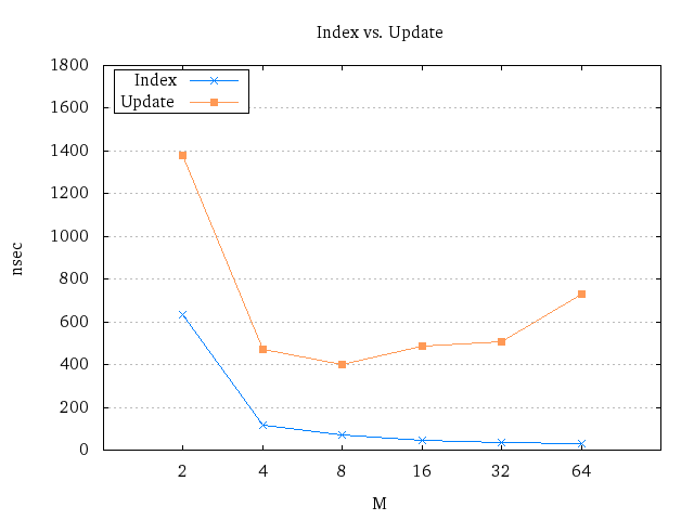
So for my master’s thesis, I did some lightweight benchmarking on the branching factor in C, on powers of 2. If you assume you will lookup elements more frequently than updating them, 32 seems like a very good fit:

The idea of fitting a node into exactly one cache line sounds neat, but unfortunately, it assumes we only have to store the pointers to our children. On the JDK, we simply cannot do that. Although there are no restrictions on how data is laid out, all the common implementations have some additional bytes in front of the object needed for polymorphism and GC. In addition, arrays need to store its length, and you need to store the transient ID somewhere as well. As a result, in OpenJDK 7, the best you can do is to store them as follows:

However, even with this overhead, the branching factor on 32 still seems to give the best tradeoff for update vs. lookup times and is still very good.

Memory

A good way to measure the memory consumption of a data structure is usually to take the memory not used on the data it stores, and divide it on the total memory used: We call this the memory overhead ratio. The lower memory overhead ratio, the better.

For array lists that doubles their capacity when they go out of space, the overhead ratio is on average 25%: At most, it will be ~50% and at best, ~0%. However, the ArrayList in Java doesn’t double its capacity, it increases it with 1.5 instead (a 100 element long array will be grown to 150). As a result, the overhead ratio for the ArrayList is actually 12.5%.

The average memory overhead for a persistent vector is a bit more difficult to compute. However, I did so in my thesis, and with the node layout shown in the previous section, we have on average 18.4% overhead. However, the overhead ratio is way more consistent, and will almost all the time be about 18.4%.

It’s worth pointing out that the overhead for both ArrayLists and the persistent vector is very good compared to other data structures in the standard Java library. For instance, the LinkedList implementation has 83.3% memory overhead (!), and the TreeMap has 80%. The lower amount of overhead also means that there’s less data stored, which again means it’s possible to store more “actual” data in the cache.

Benchmarks

But let’s get to the more interesting stuff: Benchmarks. The benchmarks themselves and the persistent vector implementation used is stored in my GitHub repository pvec-perf. The vector implementation is a bit more efficient than the Clojure implementation, but for the most part, they have the same performance characteristics. You can go to the Persistent Vector Performance blog post if you’re more interested in the differences.

To measure it against something kind-of similar and familiar, we’ll use the good old Java ArrayList (the same we just compared memory overhead ratio with – what a coincidence!). We’ll also add in transient vector benchmarks where it makes sense.

Of course, take the benchmarks with a grain of salt: These benchmarks will utilise the cache differently than your program, and performance will therefore vary.

With that in mind, let’s have a look at the plots!

Lookups

Let’s start with the obvious benchmark: Lookups. If we wanted to look up an element at a completely random index in a vector, how long would it take?

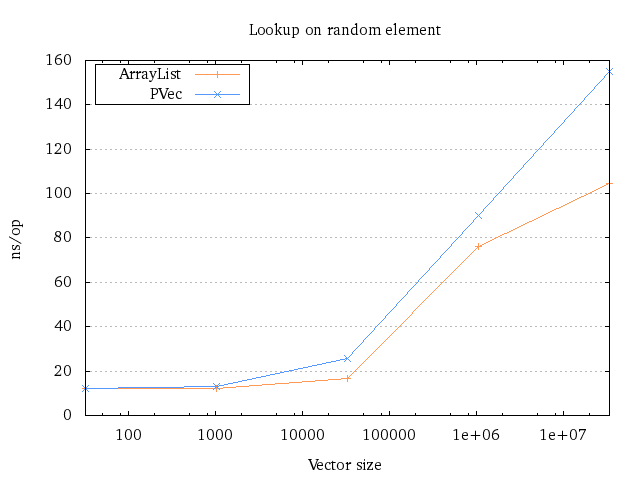
When we compare the results with the ArrayList, we see that the difference is very small, until the data structures start to contain over 1 million elements. The reason why they both increase their running time so drastically is because the cache isn’t able to keep the entire data structure in memory. Therefore, the bigger the size, the more likely it is that we have to lookup data from RAM, which is expensive.

The reason why the difference between the persistent vector and ArrayList increases from ~1 million to ~33 million is likely because a single lookup has to walk through several nodes. If multiple nodes aren’t stored in the cache, running time naturally degrades more. However, it is still able to compete pretty well – the running time isn’t even doubled.

Updates

The next question we might want to ask is how fast random updates are. Since transients speed up update operations quite significantly, it makes sense to measure those as well.

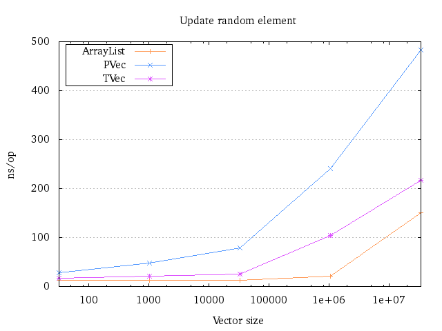
As expected, the transient is much faster than the persistent variant. What is also interesting to see is that the transient is able to compete with the ArrayList to some extent, until both start to fall out of the cache. Presumably, this penalises the transient more heavily initially, as it both has to look up a pointer AND the transient ID. The transient ID might not be stored in the same cache line, which means that every node we access might require 2 cache lines, not 1.

However, once the initial “cache pain” is over, the transients seem to fare well and reduces the gap.

Appends

Now, let’s have a look at more “complex” function: Append. We’d really like to measure the time taken to run a single append operation, but this is really hard to do right with a transient and an ArrayList: We’d have to create the transient and ArrayList all over again to get the same benchmark as if we had done a single append on the persistent variant. But at that point, you’ve changed the cache, and in the end, it will be really hard to subtract the overhead from the two other runs. Simply put, this is a big no-no for benchmark analysis.

So instead, why not measure how long time it takes to do n appends? We don’t get the running time for a single append at a specific length, but at least we can compare persistent vectors, transient vectors and ArrayLists on even ground. So we will benchmark the following code:

Coll c = new Coll();
for (int i = 0; i < n; i++) {
  c = c.append(someConstant);
}
return c;

And the results for the different data structures are as follows:

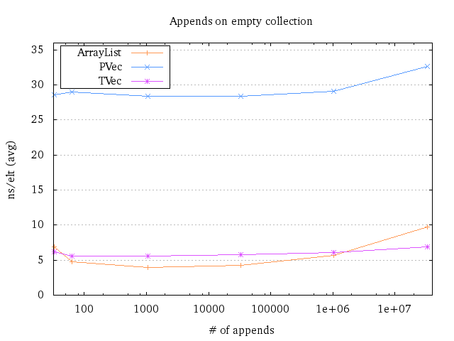
(To make sense of the results, I’ve divided the total running time by the number of elements.)

There are a lot of interesting things in this benchmark, but perhaps the biggest one is the fact that the average time for a single append is more or less constant, up until you go out of space in the cache. So, in this benchmark, appends on a persistent vector takes roughly 7 times longer than appends on an ArrayList.

The other interesting part here is the transient performance. As its persistent counterpart, the append time is constant per element. Compared to the ArrayList, it’s roughly 1.4 times slower when you can put everything into the cache. But when you can’t put everything into the cache, the transient actually beats the ArrayList!

This doesn’t necessarily mean that transients are faster in general though. I would guess transients being faster than ArrayLists in performance-tuned code will more or less never happen.

Pops

We have the same issue for popping as with appending, so we can’t measure a single pop. So instead, we’ll take a persistent version of the data structure and pop off all the elements on it. But, we can’t really measure multiple pops on the ArrayList or transient if we do this, as we’d need to create the whole data structure again. So we’re stuck with the same problem as with single appends.

However, since we are going to do multiple pops, we can make a transient out of a persistent vector and use that – which is what I have done in this benchmark. The ArrayLists are unfortunately not going to make it, because there is no way to convert an “immutable” ArrayList to a mutable one in a way that doesn’t affect the benchmark significantly.

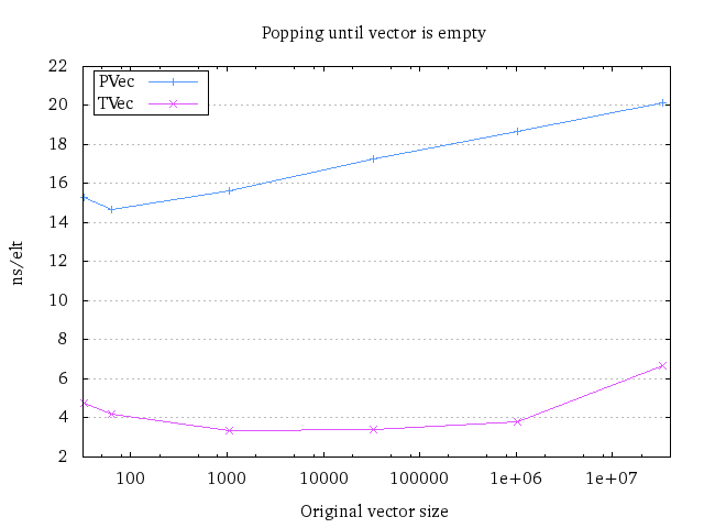
In this plot, we can easily see that pops take more time with a bigger persistent vector. However, the transient popping seems to be constant – at least the same kind of constant as ArrayList appends are. Although the difference is noticeable, the running time is much smaller than for appends (almost 10 nsec faster).

Iteration

Doing random updates and lookups isn’t that normal compared to doing a reduce or a mapv, walking the entire vector. That’s important to realise, as iterating over the complete vector can be done in O(n) time, instead of naïvely looking up each element in order, which would take O(n log n) time.

This is also relatively easy to benchmark, we just have to make sure we actually look up the values. So the benchmark does more or less this (iter):

// preparation outside of the benchmark: Create the Coll c
long sum = 0;
for (Integer val : c) {
  sum += val;
}
return sum;

Just for fun, we can measure it against the naïve version (get):

// preparation outside of the benchmark: Create the Coll c
long sum = 0;
for (int i = 0; i < size; i++) {
    sum += c.get(i);
}
return sum;

and the result we get when we do so is as follows:

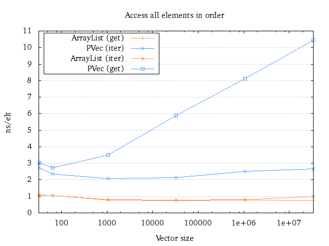
The first thing we can see is that doing the O(n) iteration technique does take constant time per element, in contrast to the get implementation which takes (a noticeable) O(log n) time per element. Iteration also seems to take roughly 3 times longer per element, compared to the ArrayList.

As a small note, it seems that doing repeated gets on an ArrayList is a tiny bit faster than doing iteration. However, the difference is so small that I don’t think it’s statistically significant.

“Full Run”

Before we wrap up, let’s have a look at a small program using these data structures in the same way. We append a bunch of (equal) values onto the data structure, iterating (reduce) over it, then pop off all the values. The code looks something like this:

Coll c = new Coll();
for (int i = 0; i < size; i++) {
  c = c.push(some_int_constant);
}
long sum = 0;
for (Object o : c) {
// or for (int i = 0; i < size; i++)
// depending on what's faster
  sum += (Integer) o;
}
for (int i = 0; i < size; i++) {
  c = c.pop();
}
return sum + c.size();

It’s not a sensible program by any means (why would you pop off all the elements?), but it’s interesting to see how the data structures compare against each other in a slightly more realistic situation.

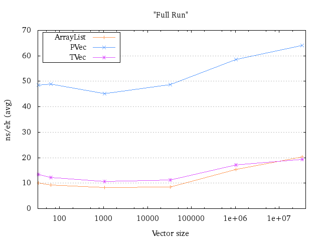
It’s clear that the transient version is very efficient, and can compete against the ArrayList very well. However, how well does the persistent variant keep up?

It keeps up amazingly well. Although it seems to increase its running time with size, you must also realise that the same happens for the ArrayList. For the smaller sizes, the persistent vector uses 5-6 times more time. That improves to only 3.8 times slower for ~1 million elements and 3.1 times slower for ~33 million elements. If anything, it seems to handle growth and shrinkage way better than the ArrayList for larger sizes.

Intuitively, this makes somewhat sense: The ArrayList has to copy all its content to another array when it has to grow. The vector implementation only has to allocate a new tail, and between 1-5 internal nodes.

Conclusion

We’ve seen the performance of the persistent vector compared to the mutable ArrayList, found in Java’s standard library. We should take benchmarks with a grain of salt, but they say the following:

• The persistent vector’s update performance is generally between 5-8x slower than an ArrayList.
• The transient vector’s update performance is comparable to the ArrayList, usually less than 1.5 times slower.
• Iteration is about 3 times slower, and lookups take no more than 2 times more time (unless the vector contains less than 1000 elements, in which case it is about just as fast).

Of course, your mileage will vary, but it’s definitely not 20-50x slower, and you shouldn’t have to worry about its performance when starting on a project¹. The persistent vector also has a very low memory overhead, only slightly higher than the average memory overhead of an ArrayList.

Now, it’s important to realise that we could specify the initial size of the ArrayList to improve its performance. That would make sense. But beating the ArrayList isn’t the point here. The point is that appends and pops on an ArrayList takes amortised O(1) time, regardless of its initial size. And – in most of the benchmarks – you cannot see which data structure is using an O(1) algorithm, and which one is using an O(log n) algorithm. The only times where the vector implementation really struggles is when there is no spatial locality (randomly uniform lookups and updates).

That the persistent vector is only a constant factor away while still using an O(log n) algorithm means that it’s not unreasonable to call its running time “effectively constant”, O(~1). The only case where this doesn’t apply is when your program is doing lookups that have very weak spatial locality, or if you have to do very HPC-like stuff. There are probably other cases as well, but the point is that you probably know if this is an issue for you already before you read this blog post.

We’ve also looked into why the persistent vector has a branching factor of 32: It’s because it currently gives the best tradeoffs between read and update times.

And with that, our adventure into the persistent vector internals ends. If you’ve read through all the blog posts in this series, you probably fully understand how the persistent vector works, how you can implement one (with optimisations), and how performant it is.