Part 1 and part 2 of this blog post series about Clojure’s persistent vectors should give you a good understanding of how the persistent vector works in general. However, there are many different ways of decreasing the constant factors. Perhaps the easiest one to grasp is the tail, which we will have a look at in this blog post.

The Rationale for Tails

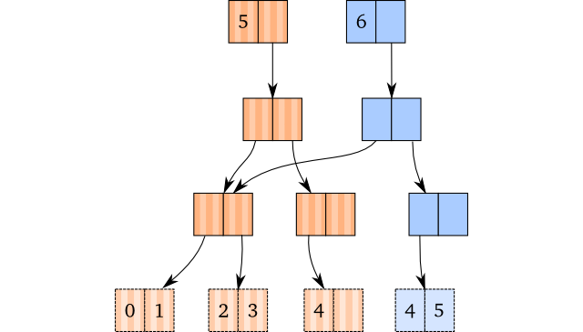
Recall that this is the visualisation of the operation (conj [1 2 3 4] 5), without any tail implemented: If there’s space in the rightmost leaf, just copy the path down to the leaf node, copy the leaf, and insert the last element into the copy.

How would this differ with a tail? Let’s have a look:

Instead of keeping the rightmost leaf in the tree itself, we keep a direct reference to it in the vector header: That’s the last block which has been added to the vector head since the last blog post. The reference to the rightmost leaf node is called the tail.

For the conj-operation, we end up checking whether there’s space in the tail. Since it is – in this case – we copy the tail and insert the new element into it. Note that this is constant time, not effectively constant time. So every time we conj onto a vector with space in its tail, we do a constant time operation.

This makes bulk operations significantly faster. If you do many conjs in a row, the result is that every operation takes on average way less time. For a vector with a branching factor of 2, 1/2 (50%) of all conj operations will (on average) be constant time. If we instead have a branching factor of 32, 31/32 of all conj operations will be actual constant time. Only 3.1% of the conj operations will be effectively constant time, meaning that we have a rather significant constant reduction. We get the same performance benefits when we perform many disjs in a row as well.

So this seems like a very attractive addition. How do we implement it?

Tail Offset

Before we look at how we implement the actual operations, we need to have a look at a very easy concept: The tail offset of a vector. We need it to be able to understand how some of the vector operations changes.

The tail offset is just the total amount of elements in the actual tree. So in practice, tail_offset = vector.length - tail.length. The reason we need the tail offset is that we sometimes need to perform the “old” operations: Looking up or modifying elements require us to know whether they are in the actual tree, or if they are in the tail.

As an example of the tail offset, consider the vectors from the previous paragraph with 5 and 6 elements. The one with 5 elements has 1 element in its tail, so its tail offset is 4. The one with 6 elements also has a tail offset of 4, as it has 2 elements in its tail.

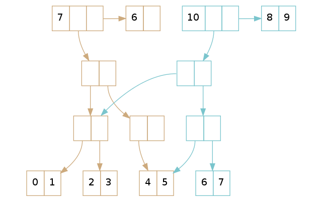
For some more examples of tail offset, look at the vectors above. The one with 7 elements in it has a tail offset of 6, and the one with 10 elements have a tail offset of 8.

Lookup

Looking up a value in a persistent vector with a tail is not too different from looking up a value in one without a tail. There are essentially two cases:

• We want to look up a value in the tail
• We want to look up a value in the tree

And here’s where we need to use the tail offset. In pseudocode, the lookup would look something like this:

if lookup_index < tail_offset:
  # tree_lookup = old lookup technique
  return tree_lookup(lookup_index)
else:
  return tail[lookup_index - tail_offset]

As we know that the tail offset is the number of elements in the tree, we can just check whether the element we are going to look up is less than the tail offset. If it is, we just do the old lookup technique. Otherwise, we know that it is in the tail. If that’s the case, we subtract the tail offset (this is why we call it the tail offset) by the index, and then look up the newly calculated index in the tail.

Update

An update is, as the lookup implementation, very similar to the original update implementation. The only difference happens when you want to update a value which resides inside the tail. We have yet again two cases: One where you update something in the tree, and something when you update the tail.

if update_index < tail_offset:
  # tree_update is the old update technique
  return tree_update(update_index, elt)
else:
  vector_copy = copy_head(this)
  vector_copy.tail = copy_tail(this.tail)
  vector_copy.tail[lookup_index - tail_offset] = elt
  return vector_copy

Let’s take a look at the case where we update something in the tree first. We can repeat the old example from part 1, where we update the element at index 5:

(def brown [0 1 2 3 4 5 6 7 8])
(def blue (assoc brown 5 'beef))

This would result in the following tree:

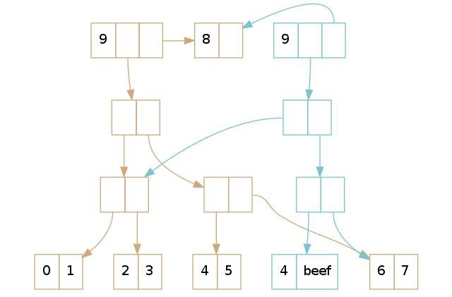
Just as in the explanation in part 1, we perform path copying and replace the element in the leaf. However, notice that they share the tail: After all, it hasn’t changed, so why bother copying it?

The second case is when we have to modify an element within the tail itself. Let’s reuse the previous example, but replace the element at index 8 instead of index 5:

(def brown [0 1 2 3 4 5 6 7 8])
(def blue (assoc brown 8 'beef))

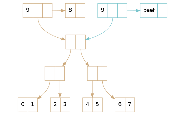
Here we see that we copy the vector “head” and the tail, and then perform the modification on it. As we haven’t done any modification on the tree, we share it with the unmodified vector. All of this takes constant time, not effectively constant time.

Insertion

Lookup and update are easy, but how would we go forward with insertion and deletion? Well, it turns out that it’s not that difficult either. For insertion, we yet again have two cases. However, they are slightly different this time around:

• We have space in the tail
• We don’t have space in the tail

The first case is – of course – easy: We just copy the tail and insert the new element at the end. The first figure in this blog post shows exactly how that works. But what do we do if there’s not enough space in the tail?

The idea is very similar to the insertion described in part 1, but with a minor modification: Instead of inserting a single value, we insert a leaf node. Recall that the tail is just a leaf node, which is directly pointed at from the root of the vector.

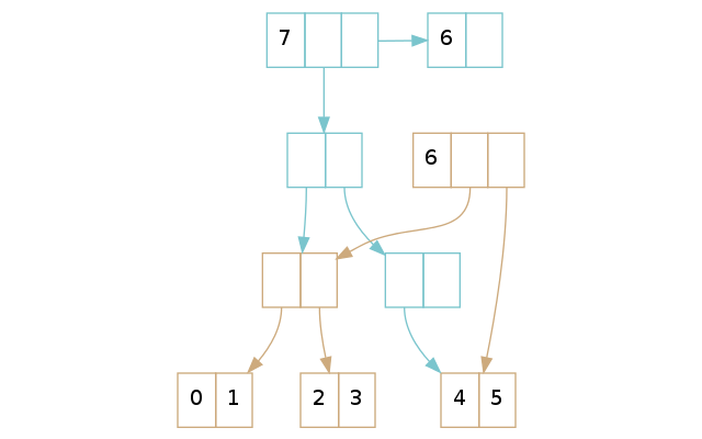
In the example above, the brown vector has a full tail: You cannot insert more elements into it. A conj on the brown vector creates the blue vector, in which we realise we must insert the tail into the tree itself. We insert the tail in the tree, using the rules from part 1, and create a new tail which we put the new element.

In effect, there’s not much more to insertion than this: It’s not difficult to grasp the understanding of it. However, an actual implementation needs to be a bit careful with indices when inserting the leaf node. Luckily, an off-by-one error is the hardest thing you’ll face if you’re implementing this.

Removal

When working on removal, we face a design choice: We have to move leaf nodes in the tree back up as tails in some cases. But when should we do it? Should we have empty tails in the persistent vector, and only move leaf nodes up as tails when we pop vectors with already empty tails? Or should we always have nonempty tails in the vector?

It turns out that there are at least two reasons for keeping the tail nonempty in all cases¹: The obvious one is that you now can guarantee that a peek is actual constant time. A more subtle one is that a random lookup will be, on average, faster: If it takes less time to look up a value in the tail than in the tree, then it is better to have a full tail than an empty one!

So, we end up – as you probably guessed – with two different cases we have to handle:

• We have more than one element in the tail
• We have one element in the tail

As I just mentioned, there won’t be any vector without elements in its tail (with the exception of the empty vector). Assuming that there is at least one element in the tail is thus perfectly fine.

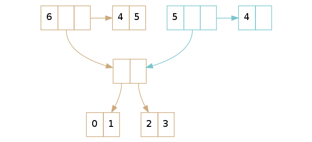
If we have more than one element in the tail, we just copy the tail, remove the last element, and return the new vector. The example above shows us that only the tail differs, which is what we would expect.

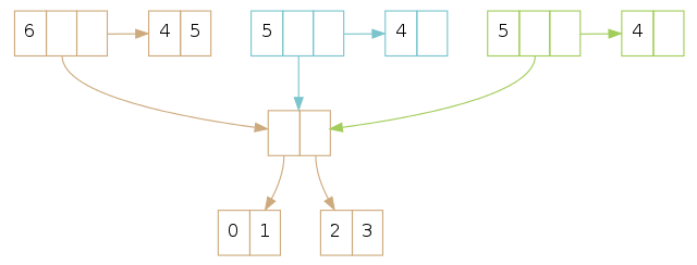
Keep in mind that if we pop on the same vector twice, we will create two tails, even though their content will be equivalent:

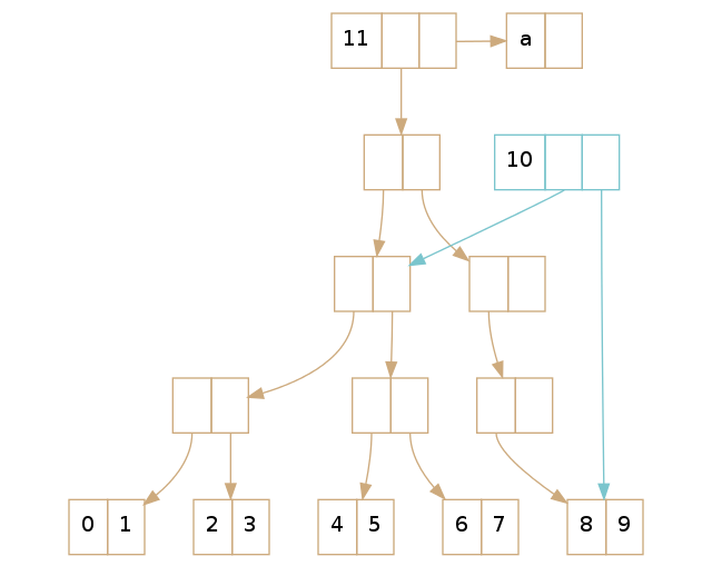
If we have a single element in the tail, we have to “promote” the rightmost leaf node in the tree as the new tail. We also have to remove it from the tree itself. Those steps are similar to looking up and popping single elements in a vector without a tail, except that you look up and pop leaf nodes instead.

The most complex example is when you have to delete empty nodes and kill the root, as further described in part 1. However, as long as you follow the rules explained there, and consider the leaf nodes to be the “elements”, you should be fine. Below is such an example, where the rightmost leaf node is “promoted” to a root node.

Next Up

The next part of this series explains transients: Why we want them and how they work. Finally, the last part of this blog post series contains a performance comparison of the ArrayList versus the persistent vector.